How and why does one conduct a landscape or riverscape genetics study?

Common methodology used for understanding how landscapes (riverscapes) influence gene flow in a species of interest relies heavily upon weighted, individual landscape features (e.g., elevation, habitat type, snow cover, or road coverage) that are combined into resistance surfaces (e.g., Spear et al., 2010). A resistance surface then becomes a hypothesis for movement (i.e., gene flow), allowing for identification of areas or barriers (Below) that imped (or enhance) gene flow. There is often no general consensus, however, on the appropriate selection and weighting scheme of landscape features.

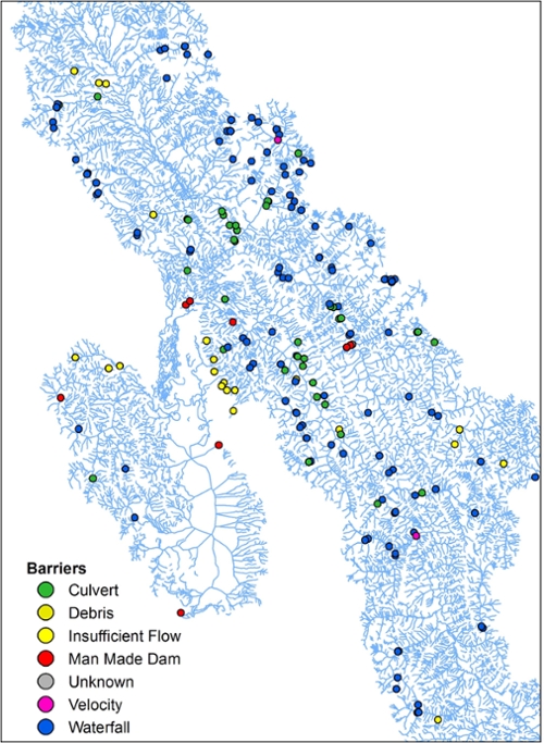
(Left) A map of the Flathead River Drainage in Montana. The map depicts barriers of various conservation impact along the river drainage. Such barriers can act to imped gene flow in a riverscape, but the relative strength of a particular barrier type may not be well known.

Terms

Gene flow -- the transfer of alleles or genes from one population to another. 

Landscape Genetics - A discipline that analyses the influence of landscape and environmental features on the genetic structure of a population.

Optimization – A search for the best fitting model or solution to a problem.

Resistance Map – A hypothesis of species dispersal based on weighted landscape variables suspected to be important to gene flow.

What is a resistance surface or map?

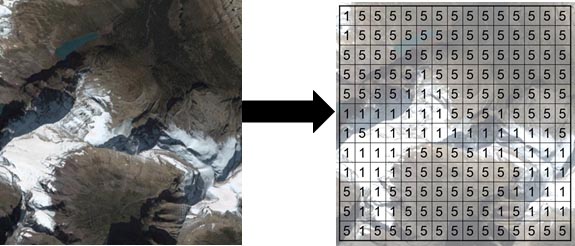
In landscape genetic studies, variables associated with features that are hypothesized to have an impact on individual movement are often represented in rasterized maps/grids. Each raster map represents some landscape or environmental variable  that can be continuous or classified data. Every pixel (small square) in a raster image can then be assigned a weight for the underlying variable (e.g., land cover can be either bare or snow-covered). Weights for each variable (across each layer) are adjusted and based on underlying gradient effects of movement, survival, abundance and reproduction (Spear et al. 2010). These weights represent the relative cost of animal movement across/through a pixel on a raster image . Finally, a resistance map is built by summing the weights associated with each variable layer (e.g. elevation, habitat type, snow) for that pixel on the map.

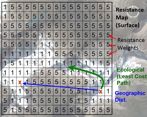
(Above) A hypothetical resistance surface or map that represents species movement (or gene flow) across the landscape where the species of interest prefers snow cover to bare landscape (e.g., Schwartz et al. 2009).  Image from Mike Schwartz.

How are the “best-fitting” resistance map weights calculated?

Once created, a hypothetical resistance surface must be run through a connectivity model to calculate effective distances (the straight line distance with any additional costs of the underlying landscape that impedes or allows gene flow). Two major connectivity models used throughout the landscape genetics literature: least-cost paths and circuit theory (Adriaensen et al. 2003; McRae 2006).

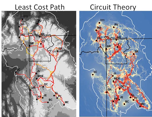
Least-cost path connectivity model

A least-cost path (Figure 3) is calculated by finding the minimum effective distance between source and destination points, (e.g., using Dijkstra's (1959) single-source shortest path algorithm; Figure 2, panel A). Least-cost modeling works partially off the general assumption that animals have perfect, or near perfect knowledge of the landscape and therefore take the shortest path when dispersing (Cushman et al. 2006; Cushman et al. 2009). For this same reason, least-cost models have been criticized for being overly simplistic (Sawyer et al. 2011).

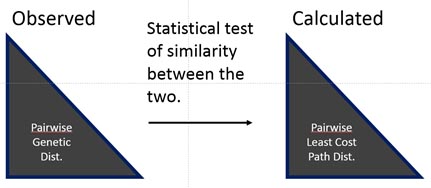
Comparing genetic structure to effective distances

To find the best-fitting resistance surface that explains genetic structure based on underlying landscape features requires running many, many (and varied) combinations  of competing resistance surfaces through a connectivity model (least-cost path or circuit theory). Resistance surfaces must then be compared in some systematic way; most often this is done using statistical tests that correlate observed pairwise genetic distances to calculated pairwise effective distances (e.g., least-cost path distances). Finally, the most highly correlated resistance maps are considered the best-fitting models of landscape features that match observed patterns of genetic connectivity!

Are there any software programs available to help? Yes, GARM is one!

By automating the process of fitting resistance maps weights to observed patterns of genetic connectivity, GARM greatly speeds up the process of resistance map creation. Further, it facilitates comparisons of many landscape variables (e.g. forest, elevation, landcover and landuse etc.) and resistance weight ranges, allowing for wide searches of landscape variable combinations in a single run. GARM can aid researchers and managers in leveraging the growing number of genetic datasets publically available to help them understand environmental variables that impede or facilitate genetic connectivity and gene flow. This leads to better understanding of species sensitivity to environmental conditions and allow for the correct inclusion of key variables in future vulnerability analyses.

References

Adriaensen F, Chardon JP, De Blust G et al. (2003) The application of “least-cost” modelling as a functional landscape model. Landscape and Urban Planning, 64, 233–247.

Cushman S, McKelvey KS, Hayden J, Schwartz MK (2006) Gene flow in complex landscapes: testing multiple hypotheses with causal modeling. The American naturalist, 168, 486–499.

Cushman S a, McKelvey KS, Schwartz MK (2009) Use of empirically derived source-destination models to map regional conservation corridors. Conservation biology : the journal of the Society for Conservation Biology, 23, 368–76.

Dijkstra EW (1959) A note on two problems in connexion with graphs. Numerische Mathematik, 1, 269–271.

McRae B (2006) Isolation by resistance. Evolution, 60, 1551–1561.

McRae BH, Dickson BG, Keitt TH, Shah VB (2008) Using circuit theory to model connectivity in ecology, evolution, and conservation. Ecology, 89, 2712–2724.

Sawyer SC, Epps CW, Brashares JS (2011) Placing linkages among fragmented habitats: do least-cost models reflect how animals use landscapes? Journal of Applied Ecology, 48, 668–678.

Schwartz MK, Copeland JP, Anderson NJ et al. (2009) Wolverine gene flow across a narrow climatic niche. Ecology, 90, 3222–32.

Spear SF, Balkenhol N, Fortin M-J, McRae BH, Scribner K (2010) Use of resistance surfaces for landscape genetic studies: considerations for parameterization and analysis. Molecular ecology, 3576–3591.